SNP Manhattan plot
[1]:
import sys; sys.path.insert(0, "../../../")
import coolbox
from coolbox.api import *
import numpy as np
[2]:
coolbox.__version__
[2]:
'0.4.0'
[3]:
data_dir = "../../../tests/test_data"
snp_file = f"{data_dir}/snp_chr9_4000000_6000000.snp"
test_region = "chr9:4000000-6000000"
SNP file:
[4]:
!head -n 5 ../../../tests/test_data/snp_chr9_4000000_6000000.snp
9       rs189401472     4000487 C       T       261481  0.00113584      -0.00280829     0.00319297      0.379119
9       rs141556758     4000942 T       G       262192  0.00131392      0.00119277      0.00296521      0.687497
9       rs117844905     4001207 A       G       262342  0.0301343       -0.000341362    0.000628006     0.586741
9       rs142341062     4002372 A       T       261738  0.00123979      6.13843e-05     0.003055        0.983969
9       rs500044        4002823 G       A       262342  0.131891        0.000325518     0.000317269     0.304892
Specify the column names of the input file:
[7]:
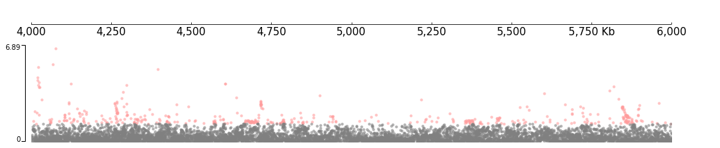
frame = XAxis() + SNP(snp_file, fields=["chrom", "rsid", "pos", "a1", "a2", "n", "maf", "beta", "se", "pval"])
frame.plot(test_region)
[7]:
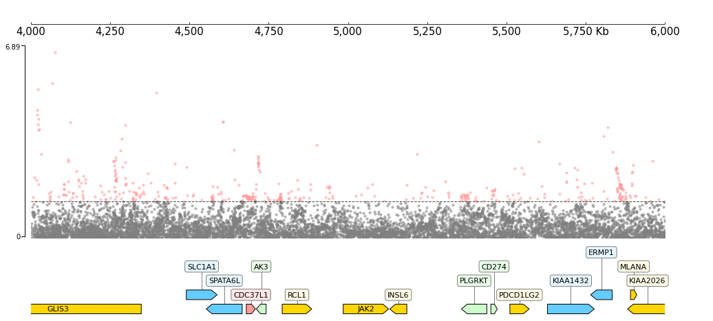
Plot with genes:
[9]:
gtf_file = f"{data_dir}/gtf_chr9_4000000_6000000.gtf"

frame = XAxis() + \
    SNP(snp_file, col_chrom=0, col_pos=2, col_pval=9) + TrackHeight(10) + HLines(-np.log10(0.05)) + \
    GTF(gtf_file)

frame.plot(test_region)
[9]:
CLI code
[10]:
%%bash

snp_file="../../../tests/test_data/snp_chr9_4000000_6000000.snp"
gtf_file="../../../tests/test_data/gtf_chr9_4000000_6000000.gtf"

coolbox add XAxis - \
add SNP $snp_file --col_chrom 0 --col_pos 2 --col_pval 9 - \
add TrackHeight 10 - \
add GTF $gtf_file - \
goto "chr9:4000000-6000000" - \
plot /tmp/test_coolbox.png