DNA features

import coolbox
from coolbox.api import *

coolbox.__version__

'0.4.0'

test_data_dir = "../../../tests/test_data/"
test_interval = "chr9:4500000-5500000"
example_bed6 = f"{test_data_dir}/bed6_chr9_4000000_6000000.bed"
example_bed9 = f"{test_data_dir}/bed9_chr9_4000000_6000000.bed"
example_bed12 = f"{test_data_dir}/bed_chr9_4000000_6000000.bed"
example_tad = f"{test_data_dir}/tad_chr9_4000000_6000000.bed"

BED file

gene style

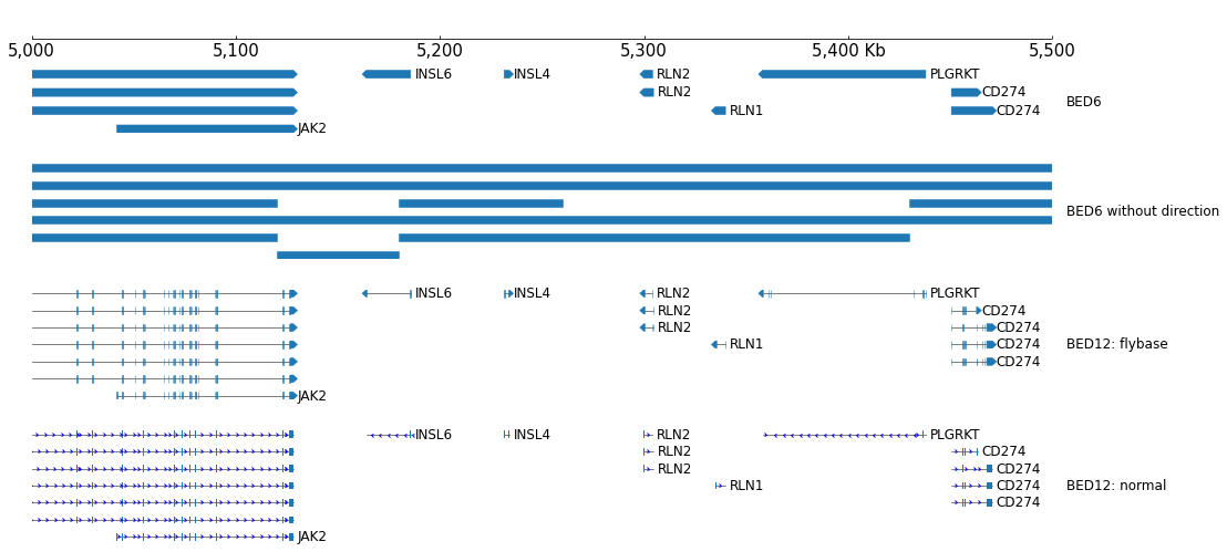
BED12 format can plot fish-bone like shapes, BED6 and BED9 can not:

frame = XAxis()
frame += BED(example_bed6) + Title("BED6")
frame += Spacer(1) +  BED(example_tad, labels=False) + Title("BED6 without direction")
frame += Spacer(1) + BED(example_bed12, gene_style='flybase') + Title("BED12: flybase")
frame += Spacer(1) + BED(example_bed12, gene_style='normal') + Title("BED12: normal")
frame.plot("chr9:5000000-5500000")

layout

The default height of BED is 'auto', it means the height is auto-growth, we can set the heigh of one row by the row_height parameter:

frame = XAxis() + BED(example_bed12, row_height=1.0)
frame.plot(test_interval)

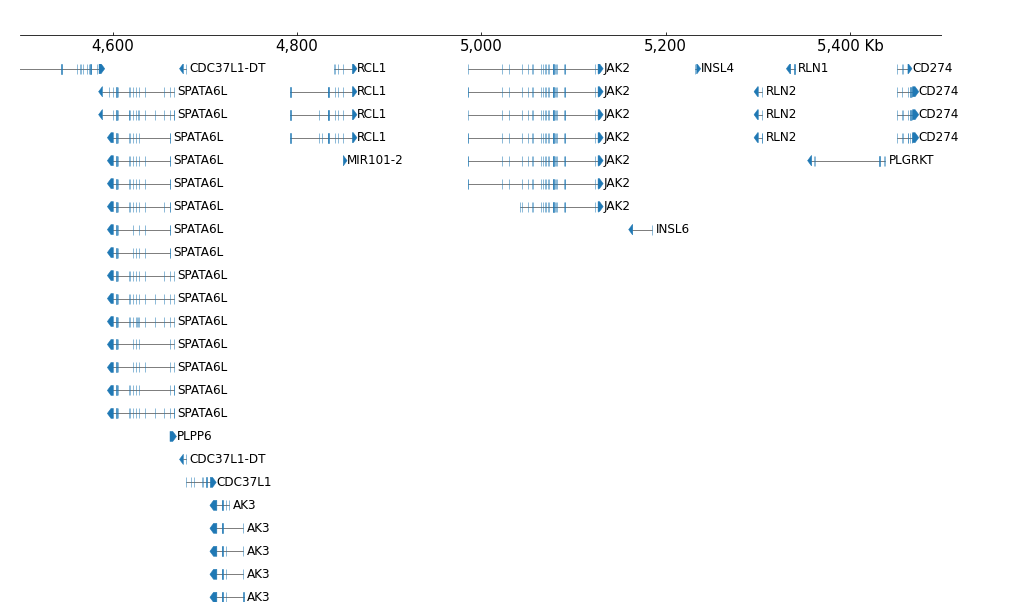
If you want fixed track height, just specify with 'height' parameter:

frame = XAxis() + BED(example_bed12, height=8, fontsize=10)
frame.plot(test_interval)

The number of rows to display can be limited by setting num_rows parameter:

frame = XAxis() + BED(example_bed12, row_height=1.0, num_rows=5)
frame.plot(test_interval)

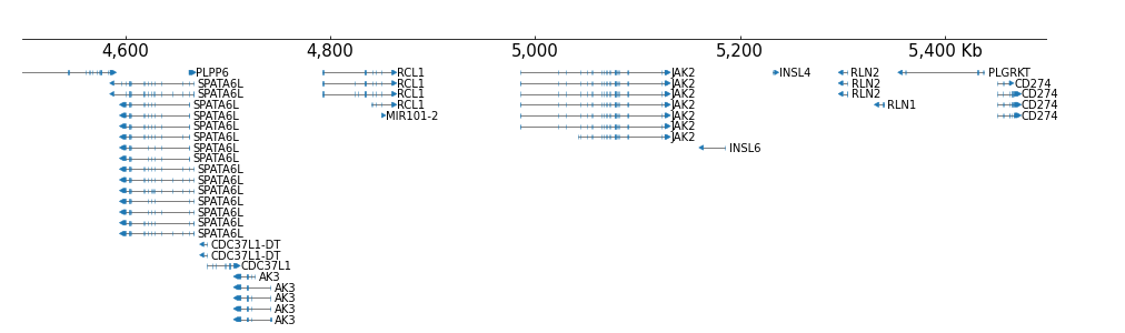
And rows can be collapsed:

frame = XAxis() + BED(example_bed12, display='collapsed')
frame.plot("chr9:5000000-5500000")

This can used for visualize the ChromStates:

frame = XAxis() + BED(f"{test_data_dir}/bed_chr9_4000000_6000000_chromstates.bed", display='collapsed') + TrackHeight(0.6)
frame.plot("chr9:5000000-5500000")

bed = BED(f"{test_data_dir}/bed_chr9_4000000_6000000_chromstates.bed", display='collapsed')

bed.fetch_data(GenomeRange("chr9:5000000-5500000"))

	chrom	start	end	name	score	strand	thick_start	thick_end	rgb
0	chr9	4996201	5004200	11_Weak_Txn	0.0	.	4996200	5004200	153,255,102
1	chr9	5004201	5005000	10_Txn_Elongation	0.0	.	5004200	5005000	0,176,80
2	chr9	5005001	5005200	15_Repetitive/CNV	0.0	.	5005000	5005200	245,245,245
3	chr9	5005201	5012600	11_Weak_Txn	0.0	.	5005200	5012600	153,255,102
4	chr9	5012601	5018600	10_Txn_Elongation	0.0	.	5012600	5018600	0,176,80
...	...	...	...	...	...	...	...	...	...
86	chr9	5497401	5497600	7_Weak_Enhancer	0.0	.	5497400	5497600	255,252,4
87	chr9	5497601	5499000	11_Weak_Txn	0.0	.	5497600	5499000	153,255,102
88	chr9	5499001	5499600	7_Weak_Enhancer	0.0	.	5499000	5499600	255,252,4
89	chr9	5499601	5499800	5_Strong_Enhancer	0.0	.	5499600	5499800	250,202,0
90	chr9	5499801	5500800	4_Strong_Enhancer	0.0	.	5499800	5500800	250,202,0

91 rows × 9 columns

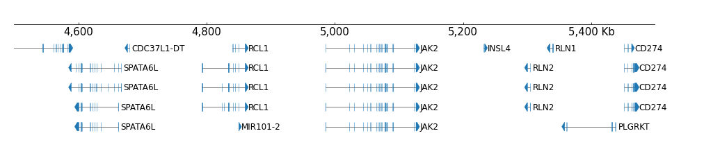
GTF file

In default GTF only plot genes with dna-feature-viewer.

example_gtf = f"{test_data_dir}/gtf_chr9_4000000_6000000.gtf"
frame = XAxis() + GTF(example_gtf) + Title("Genes")
frame.plot(test_interval)

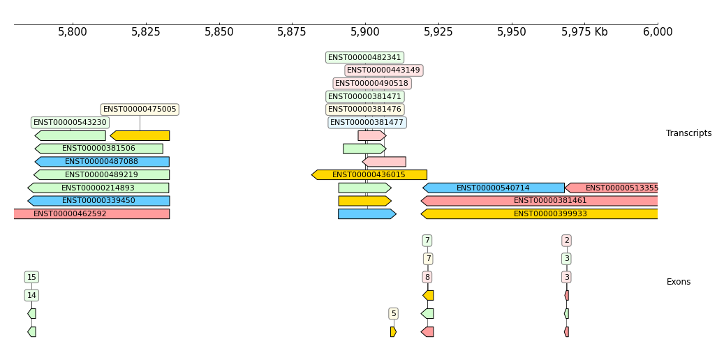
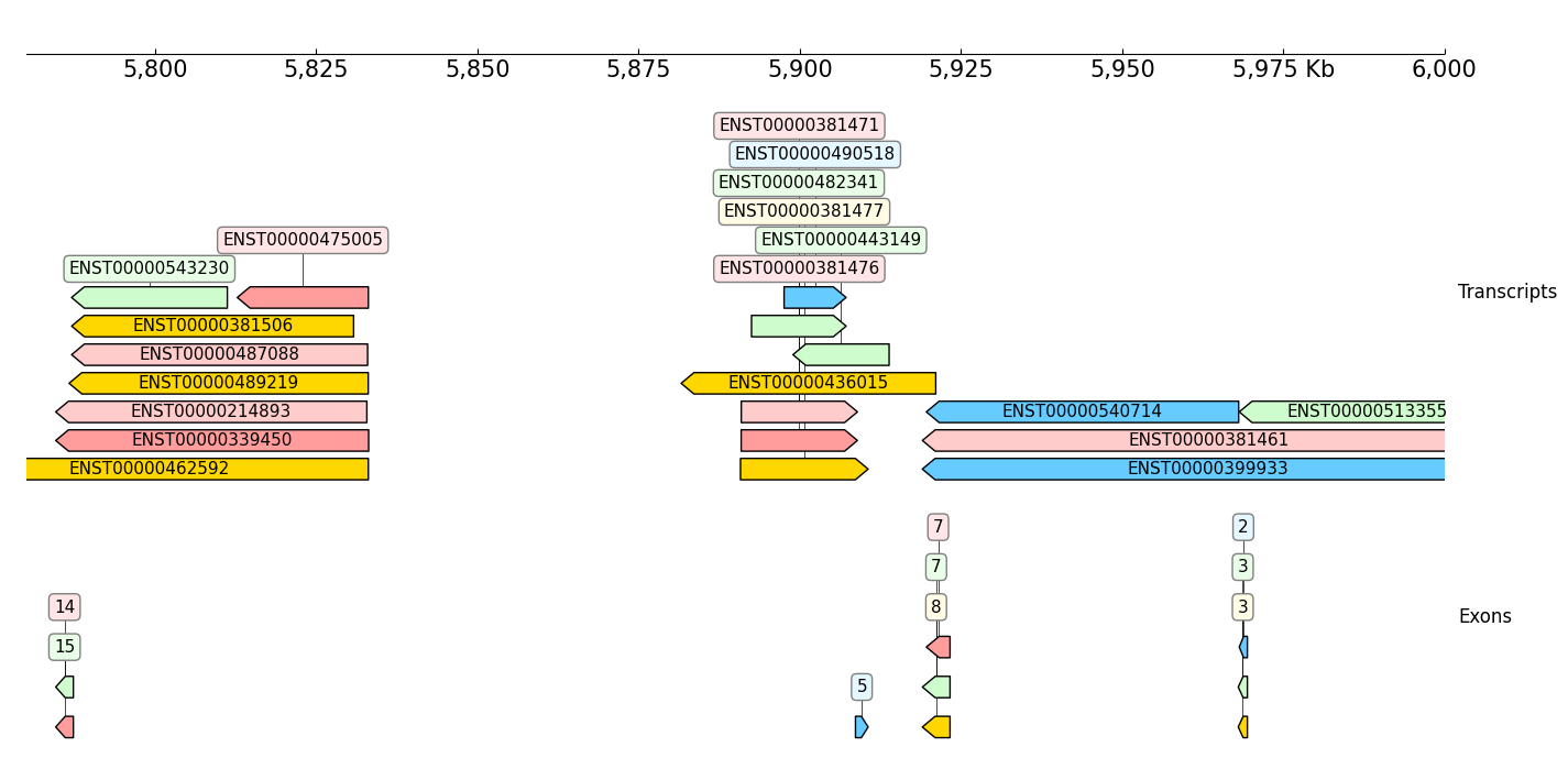
Show transcripts and exons, 'name_attr' controls show which attribute:

frame = XAxis()
frame += GTF(example_gtf, row_filter="type == 'transcript'", name_attr='transcript_id') + TrackHeight(9) + Title("Transcripts")
frame += GTF(example_gtf, row_filter="type == 'exon'", name_attr='exon_number') + TrackHeight(6) + Title("Exons")
frame.plot("chr9:5780000-6000000")

Attribute means the features in the attribute columns of the GTF:

gtf = GTF(example_gtf)
df = gtf.fetch_data(GenomeRange(test_interval))
df.head(2)

	seqname	source	type	start	end	score	strand	frame	attributes	feature_name
0	chr9	protein_coding	gene	4490444	4587469	NaN	+	NaN	gene_biotype "protein_coding"; gene_id "ENSG00...	SLC1A1
1	chr9	protein_coding	transcript	4490444	4587469	NaN	+	NaN	ccds_id "CCDS6452"; gene_biotype "protein_codi...	SLC1A1

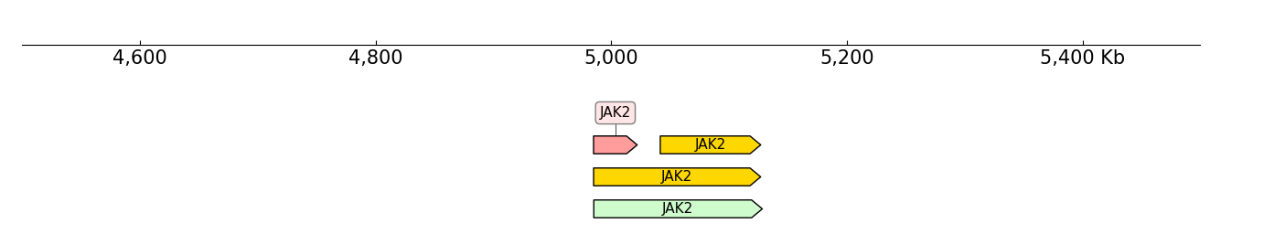
row filter can also filter the rows by other columns, for example only show the transcripts from JAK2 gene:

frame = XAxis()
frame += GTF(example_gtf, row_filter="type == 'transcript';feature_name == 'JAK2'")
frame.plot(test_interval)