Customizing CoolBox
This document is talking about how to create user-defined Track and Coverage types.
Interactive online version: Binder
CoolBox provided a lot of builtin Track and Coverage types for different kinds of genomic data formats and display form. But maybe these can’t cover all your needs some time.
The good news is that, it’s very easy to define new element types(Track, Coverage, Feature) in CoolBox!
The CoolBox plot system is compitible with matplotlib Python library, you only need to know some basic usage of it.
[1]:
# firstly import the coolbox, and check the version:
import sys; sys.path.insert(0, "../")
import coolbox
from coolbox.api import *
coolbox.__version__
[1]:
'0.3.1'
Custom Track
To implement a new Track, the only three thing you need to do:
Import the base
Trackclass fromcoolbox.core.basemodule.Create new track type, and inherit the
Trackas parent class.Implement the
plotandfetch_data(optional) method.
The code schema will look like this:
from coolbox.core.Track.base import Track

class MyTrack(Track):
    def __init__(self, ...):
        # Initialization
        pass

    def plot(self, ax, genome_range, *kwargs):
        # Method for plot the track
        # within the genome range "chrom:start-end". `genome_range` is a `GenomeRange` object with properties: chrom, start, end
        # Draw in the pass-in `ax` Axes
        pass

    def fetch_data(self, genome_range, **kwargs):
        # Method for fetch the data within genome_range
        # genome_range is a `coolbox.utilities.GenomeRange` object
        pass
For better understand it, here we give an example of two simple toy tracks defination:
Chromosome name track
We can define a simple track to show the chromesome name:
[2]:
from coolbox.core.track.base import Track
from coolbox.utilities import to_gr
import matplotlib.pyplot as plt

class ChromName(Track):
    def __init__(self, fontsize=50, offset=0.45):
        super().__init__({
            "fontsize": fontsize,
            "offset": offset,
        })  # init Track class

    def fetch_data(self, gr, **kwargs):
        return gr.chrom  # return chromosome name

    def plot(self, ax, gr, **kwargs):
        x = gr.start + self.properties['offset'] * (gr.end - gr.start)
        ax.text(x, 0, gr.chrom, fontsize=self.properties['fontsize'])
        ax.set_xlim(gr.start, gr.end)
[3]:
frame = ChromName() + XAxis()
frame.plot("chr9:4000000-6000000")
[3]:
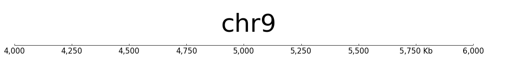
As shown above, we defined a chromesome name display track with just abouot 20 lines of Python code.
Pokemon track
Here we have a more interesting demo:
For example we want to plot some pokemons on some genome regions, and we have a BED like text file like this:
chr1    1000    2000    Bulbasaur
chr1    2000    3000    Charmander
chr1    3000    4000    Squirtle
chr1    4000    5000    Pikachu
We stores it in ./_static/pokemons/list.txt.
[4]:
!ls ./_static/pokemons
Bulbasaur.png  Pikachu.png    Squirtle.png
Charmander.png PokeBall.png   list.txt
[5]:
from coolbox.core.track.base import Track
from coolbox.utilities import to_gr
import pandas as pd
import matplotlib.pyplot as plt
from matplotlib.offsetbox import OffsetImage, AnnotationBbox

class Pokemon(Track):

    def __init__(self, file, img_dir):
        # read the table
        self.df = pd.read_csv(file, sep="\t", header=None)
        self.df.columns = ['chrom', 'start', 'end', 'pokemon']
        # directory store the images
        self.img_dir = img_dir
        super().__init__({})  # init Track class

    def fetch_data(self, genome_range, **kwargs):
        gr = to_gr(genome_range) # force convert to GenomeRange object
        df = self.df
        sub_df = df[
            (df['chrom'] == gr.chrom) & (df['start'] >= gr.start) & (df['end'] <= gr.end)
        ]
        return sub_df

    def plot(self, ax, gr, **kwargs):
        df = self.fetch_data(f"{gr.chrom}:{gr.start}-{gr.end}")  # get data in range
        for _, row in df.iterrows():
            img_path = f"{self.img_dir}/{row['pokemon']}.png" # get image path
            im = plt.imread(img_path)
            oi = OffsetImage(im, zoom = 0.5)
            px = (row['start'] + row['end']) / 2  # X position
            py = 0
            box = AnnotationBbox(oi, (px, py), frameon=False)
            ax.add_artist(box)
        ax.set_xlim(gr.start, gr.end)
        ax.set_ylim(-1, 1)
[6]:
pkm = Pokemon("./_static/pokemons/list.txt", "./_static/pokemons/")
frame = XAxis() + Spacer() + pkm
[7]:
# Fetch region data
pkm.fetch_data("chr1:0-6000")
[7]:
| chrom | start | end | pokemon | |
|---|---|---|---|---|
| 0 | chr1 | 1000 | 2000 | Bulbasaur |
| 1 | chr1 | 2000 | 3000 | Charmander |
| 2 | chr1 | 3000 | 4000 | Squirtle |
| 3 | chr1 | 4000 | 5000 | Pikachu |
[8]:
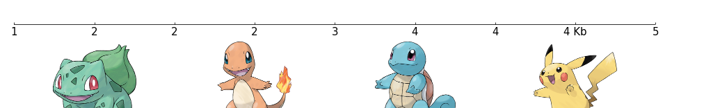
# plot region
frame.plot("chr1:1000-5000")
[8]:
Custom Coverage
Coverage is a layer draw upon the track. Custom Coverage defination is same to the Track, just define the plot and fetch_data (optional) method.
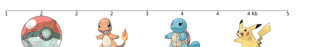
For example we can define a Poke Ball Coverage to draw upon Pokemon Track:
[9]:
from coolbox.core.coverage.base import Coverage
from coolbox.utilities import GenomeRange

pokeball_path = "./_static/pokemons/PokeBall.png"

class PokeBall(Coverage):
    def __init__(self, genome_range, img_path=pokeball_path, alpha=0.5):
        super().__init__({
            "genome_range": GenomeRange(genome_range),
            "img_path": img_path,
            "alpha": alpha,
        })

    def plot(self, ax, gr, **kwargs):
        gr = self.properties['genome_range']
        img_path = self.properties['img_path']
        alpha = self.properties['alpha']
        im = plt.imread(img_path)
        oi = OffsetImage(im, zoom = 0.8, alpha=alpha)
        px = (gr.start + gr.end) / 2  # X position
        box = AnnotationBbox(oi, (px, 0), frameon=False)
        ax.add_artist(box)
[10]:
pkm = Pokemon("./_static/pokemons/list.txt", "./_static/pokemons/")
ball = PokeBall("chr1:1000-2000", alpha=0.6)
frame = XAxis() + Spacer() + pkm + ball
[11]:
frame.plot("chr1:1000-5000")
[11]:
Coverage’s related Track is stored at it’s .track attribute:
[12]:
ball.track
[12]:
<__main__.Pokemon at 0x7fdd82838100>
Maybe you found that track defination is almost same to Track. Actually you can create a Coverage directly from Track class, by using track_to_coverage function, for example, we convert our ChromName Track to Coverage:
[13]:
from coolbox.core.coverage.base import track_to_coverage

ChromNameCov = track_to_coverage(ChromName)
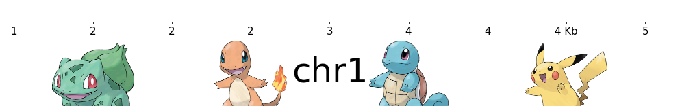
Let’s plot a chromosome name upon pokemon track:
[14]:
pkm = Pokemon("./_static/pokemons/list.txt", "./_static/pokemons/")
frame = XAxis() + Spacer() + pkm + ChromNameCov(offset=0.44)
frame.plot("chr1:1000-5000")
[14]:
Custom Feature
Feature object is used for modify Track or Coverage’s properties (like color, track height, …), for example modify track’s color:
[15]:
bigwig_path = "../../tests/test_data/bigwig_chr9_4000000_6000000.bw"

bw = BigWig(bigwig_path)
frame = XAxis() + bw + Color("#ff0c0c")
frame.plot("chr9:4000000-6000000")
[15]:
We can define our own color Feature:
[16]:
from coolbox.core.feature import Feature

class MyColor(Feature):
    def __init__(self, value):
        super().__init__(color=value)
[17]:
bw = BigWig(bigwig_path)
frame = XAxis() + bw + MyColor("#0c0cff")
frame.plot("chr9:4000000-6000000")
[17]:
Actually, all properties of CoolBox builtin tracks and coverages is stored in the .properties attribute, it’s a dict object. Add Feature is equivalent to modify this dict:
[18]:
bw.properties
[18]:
{'height': 2,
 'color': '#0c0cff',
 'name': 'BigWig.2',
 'title': '',
 'style': 'fill',
 'fmt': '-',
 'line_width': 2.0,
 'size': 10,
 'threshold_color': '#ff9c9c',
 'threshold': inf,
 'cmap': 'bwr',
 'alpha': 1.0,
 'orientation': None,
 'data_range_style': 'y-axis',
 'min_value': 'auto',
 'max_value': 'auto',
 'type': 'line',
 'num_bins': 700,
 'file': '../../tests/test_data/bigwig_chr9_4000000_6000000.bw'}
[19]:
bw.properties['color'] = "#9c5f2c"
frame = XAxis() + bw
frame.plot("chr9:4000000-6000000")
[19]:

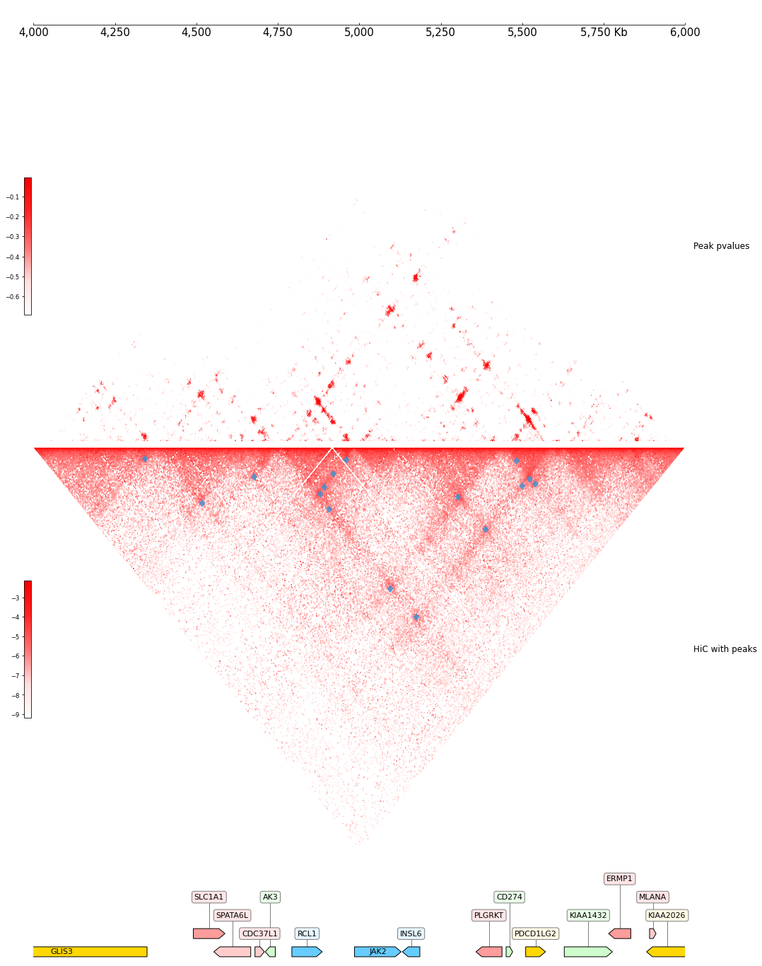
Peakachu
This document shows the ability of cooperating with newly developed algorithms. Peakachu is an machine-learning algorithm used for detecting loops in hic contact matrix.
With the user-friendly plotting and data-fetching api supplied by CoolBox, we can quickly visualize the outputs of Peakachu along with other builtin tracks in CoolBox.
install peakachu
download pretrained model listed in Peakachu
[20]:
!pip install Scikit-learn==0.22 joblib==0.14
!pip install peakachu
Requirement already satisfied: Scikit-learn==0.22 in /Users/bakezq/opt/miniconda3/lib/python3.8/site-packages (0.22)
Requirement already satisfied: joblib==0.14 in /Users/bakezq/opt/miniconda3/lib/python3.8/site-packages (0.14.0)
Requirement already satisfied: scipy>=0.17.0 in /Users/bakezq/opt/miniconda3/lib/python3.8/site-packages (from Scikit-learn==0.22) (1.5.4)
Requirement already satisfied: numpy>=1.11.0 in /Users/bakezq/opt/miniconda3/lib/python3.8/site-packages (from Scikit-learn==0.22) (1.19.4)
Requirement already satisfied: peakachu in /Users/bakezq/opt/miniconda3/lib/python3.8/site-packages (1.1.3)
Define custom track
[21]:
import joblib
import pandas as pd
from scipy.sparse import coo_matrix
from peakachu.scoreUtils import Chromosome
from peakachu import peakacluster
from coolbox.api import *
from coolbox.core.track.hicmat import Cool
from coolbox.utilities import GenomeRange, correspond_track

model = joblib.load('../../tests/test_data/down100.ctcf.pkl')


class Peakachu(Cool):
    def __init__(self, *args, **kwargs):
        super().__init__(*args, **kwargs)

    def fetch_data(self, genome_range1, **kwargs):
        matrix = super().fetch_data(genome_range1, **kwargs) # reuse Cool.fetch_data to get the raw contacts
        ch = Chromosome(coo_matrix(matrix), model) # call peakachu
        pval_ma, raw_ma = ch.score()
        self.pval_ma = pval_ma.tocoo()
        # should return a np.ndarray representing matrix
        return (pval_ma + pval_ma.T).toarray()

@track_to_coverage
class PeakaChuLoops(ArcsBase):
    def __init__(self, peakachu, **kwargs):
        super().__init__(style="hicpeaks", **kwargs)
        peakachu = correspond_track(peakachu)
        self.peakachu = peakachu

    def fetch_data(self, gr: GenomeRange, **kwargs):
        ma = self.peakachu.pval_ma
        mask = ma.data > 0.87 # threshold to filter pvals
        pixels = dict(zip(zip(ma.row[mask], ma.col[mask]), 1 / ma.data[mask]))
        rows = [(x, x + 1, y, y + 1) # call peakachu
                for [x, y], *_ in peakacluster.local_clustering(pixels, res=10000)]
        # should return a pd.DataFrame with columns ['start1', 'end1', 'start2', 'end2']
        peaks = pd.DataFrame(rows, columns=['start1', 'end1', 'start2', 'end2']) * self.peakachu.fetched_binsize + gr.start
        return peaks
Visualize Track
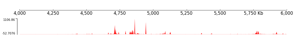
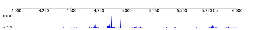
[22]:
DATA_DIR = "../../tests/test_data"
TEST_RANGE = "chr9:4000000-6000000"
RANGE_MARK = "chr9_4000000_6000000"
COOL_PATH = f"{DATA_DIR}/cool_{RANGE_MARK}.mcool"

PVALS = Peakachu(COOL_PATH, style="triangular")
PEAKS = Cool(COOL_PATH, style="triangular", orientation="inverted") + \
        PeakaChuLoops(PVALS, line_width=5)

frame = XAxis() + \
    PVALS + Title("Peak pvalues") + \
    PEAKS + Title("HiC with peaks") + \
    Spacer(0.5) + \
    GTF(f"{DATA_DIR}/gtf_{RANGE_MARK}.gtf") + TrackHeight(5)

frame.plot(TEST_RANGE)
scoring matrix chrm
num candidates 79800
[22]:
CLI Mode
Custom elements can also used in CLI mode, just save your definition to a .py file, and load_module in CLI:
[23]:
%%bash
module_path=./_static/peakachu_track.py
data_dir=../../tests/test_data/
cool_path=$data_dir/cool_chr9_4000000_6000000.mcool
gtf_path=$data_dir/gtf_chr9_4000000_6000000.gtf

coolbox load_module $module_path - \
    add XAxis - \
    add Peakachu $cool_path --style "triangular" --name "pvals" - \
    add Cool $cool_path --style "triangular" --orientation "inverted" - \
    add PeakaChuLoops "pvals" --line_width 5 -\
    add GTF $gtf_path --height 5 - \
    goto "chr9:4000000-6000000" - \
    plot "/tmp/test_coolbox_peakachu.pdf"
scoring matrix chrm
num candidates 79800
Browser Mode
Custom elements are naturally adaptive to browser mode. For use custom tracks defined above, just run:
[24]:
bsr = Browser(frame)
bsr.goto(TEST_RANGE)
bsr.show()
scoring matrix chrm
num candidates 80200