Quickstart (API)
This document is for teaching the basic usage of coolbox API and explaining some basic conceptions. It is a good starting point for using CoolBox.
Interactive online version: Binder
First, let’s import all the components from coolbox.api, and check your CoolBox version.
[1]:
# change working directory
import os
os.chdir("../../")
print(f"Current working directory: {os.path.abspath(os.curdir)}")
Current working directory: /mnt/c/Users/wzxu/Desktop/CoolBox
[2]:
import coolbox
from coolbox.api import *
[3]:
coolbox.__version__
[3]:
'0.4.0'
Data preparation
Testing dataset
Here, we use a small testing dataset for convenience. This dataset contains files in differnet file formats, and they are in the same genome range (chr9:4000000-6000000) of the human reference genome (hg19).
[4]:
!pwd
!ls -lh tests/test_data/
/mnt/c/Users/wzxu/Desktop/CoolBox
total 99M
-rwxrwxrwx 1 wzxu wzxu 787K Feb 26  2025 bam_chr9_4000000_6000000.bam
-rwxrwxrwx 1 wzxu wzxu 5.8K Nov  4 23:13 bam_chr9_4000000_6000000.bam.bai
-rwxrwxrwx 1 wzxu wzxu 1.5K Feb 26  2025 bed6_chr9_4000000_6000000.bed
-rwxrwxrwx 1 wzxu wzxu  449 Nov  4 23:10 bed6_chr9_4000000_6000000.bed.bgz
-rwxrwxrwx 1 wzxu wzxu  220 Nov  4 23:10 bed6_chr9_4000000_6000000.bed.bgz.tbi
-rwxrwxrwx 1 wzxu wzxu 2.3K Feb 26  2025 bed9_chr9_4000000_6000000.bed
-rwxrwxrwx 1 wzxu wzxu 8.6K Feb 26  2025 bed_chr9_4000000_6000000.bed
-rwxrwxrwx 1 wzxu wzxu 2.0K Nov  4 23:10 bed_chr9_4000000_6000000.bed.bgz
-rwxrwxrwx 1 wzxu wzxu  226 Nov  4 23:10 bed_chr9_4000000_6000000.bed.bgz.tbi
-rwxrwxrwx 1 wzxu wzxu  34K Feb 26  2025 bed_chr9_4000000_6000000_chromstates.bed
-rwxrwxrwx 1 wzxu wzxu 5.0K Nov  4 23:10 bed_chr9_4000000_6000000_chromstates.bed.bgz
-rwxrwxrwx 1 wzxu wzxu  399 Nov  4 23:10 bed_chr9_4000000_6000000_chromstates.bed.bgz.tbi
-rwxrwxrwx 1 wzxu wzxu  19K Feb 26  2025 bedgraph_chr9_4000000_6000000.bg
-rwxrwxrwx 1 wzxu wzxu 4.1K Nov  4 23:13 bedgraph_chr9_4000000_6000000.bg.bgz
-rwxrwxrwx 1 wzxu wzxu 4.5K Nov  4 23:13 bedgraph_chr9_4000000_6000000.bg.bgz.tbi
-rwxrwxrwx 1 wzxu wzxu  270 Feb 26  2025 bedpe_chr9_4000000_6000000.bedpe
-rwxrwxrwx 1 wzxu wzxu  149 Nov  4 23:09 bedpe_chr9_4000000_6000000.bedpe.bgz
-rwxrwxrwx 1 wzxu wzxu  158 Nov  9 19:53 bedpe_chr9_4000000_6000000.bedpe.bgz.px2
-rwxrwxrwx 1 wzxu wzxu  366 Feb 26  2025 bedpe_var_chr9_4000000_6000000.bedpe
-rwxrwxrwx 1 wzxu wzxu  165 Nov  4 23:23 bedpe_var_chr9_4000000_6000000.bedpe.bgz
-rwxrwxrwx 1 wzxu wzxu  173 Nov  9 19:53 bedpe_var_chr9_4000000_6000000.bedpe.bgz.px2
-rwxrwxrwx 1 wzxu wzxu  31K Feb 26  2025 bigwig_chr9_4000000_6000000.bw
-rwxrwxrwx 1 wzxu wzxu 158K Feb 26  2025 bigwig_chr9_4000000_6000000_K562_H3K27ac.bigwig
-rwxrwxrwx 1 wzxu wzxu 240K Feb 26  2025 bigwig_chr9_4000000_6000000_K562_H3K27me3.bigwig
-rwxrwxrwx 1 wzxu wzxu 452K Feb 26  2025 bigwig_chr9_4000000_6000000_K562_H3K4me3.bigwig
-rwxrwxrwx 1 wzxu wzxu 124K Feb 26  2025 bigwig_chr9_4000000_6000000_K562_RNA.bigwig
-rwxrwxrwx 1 wzxu wzxu  62K Feb 26  2025 chr9.1.pc.bedGraph
-rwxrwxrwx 1 wzxu wzxu  20K Nov  4 23:11 chr9.1.pc.bedGraph.bgz
-rwxrwxrwx 1 wzxu wzxu 3.5K Nov  4 23:11 chr9.1.pc.bedGraph.bgz.tbi
-rwxrwxrwx 1 wzxu wzxu  24M Feb 26  2025 cool_chr1_89000000_90400000_for_cmp_1.mcool
-rwxrwxrwx 1 wzxu wzxu  23M Feb 26  2025 cool_chr1_89000000_90400000_for_cmp_2.mcool
-rwxrwxrwx 1 wzxu wzxu  27M Feb 26  2025 cool_chr9_4000000_6000000.mcool
-rwxrwxrwx 1 wzxu wzxu  14M Feb 26  2025 dothic_chr9_4000000_6000000.hic
-rwxrwxrwx 1 wzxu wzxu 9.3M Feb 26  2025 down100.ctcf.pkl
-rwxrwxrwx 1 wzxu wzxu 537K Feb 26  2025 gtf_chr9_4000000_6000000.gtf
-rwxrwxrwx 1 wzxu wzxu  27K Nov  4 23:10 gtf_chr9_4000000_6000000.gtf.bgz
-rwxrwxrwx 1 wzxu wzxu  398 Nov  4 23:10 gtf_chr9_4000000_6000000.gtf.bgz.tbi
-rwxrwxrwx 1 wzxu wzxu 537K Feb 26  2025 gtf_chr9_4000000_6000000_fake.gtf
-rwxrwxrwx 1 wzxu wzxu  34K Feb 26  2025 hg19_ideogram.txt
-rwxrwxrwx 1 wzxu wzxu 6.7K Nov  9 19:37 hg19_ideogram.txt.bgz
-rwxrwxrwx 1 wzxu wzxu 8.5K Nov  9 19:37 hg19_ideogram.txt.bgz.tbi
-rwxrwxrwx 1 wzxu wzxu 2.1K Feb 26  2025 human.hg19.genome
-rwxrwxrwx 1 wzxu wzxu 3.1K Feb 26  2025 make_test_dataset.py
-rwxrwxrwx 1 wzxu wzxu  799 Feb 26  2025 pairs_chr9_4000000_6000000.pairs
-rwxrwxrwx 1 wzxu wzxu  292 Nov  4 23:09 pairs_chr9_4000000_6000000.pairs.bgz
-rwxrwxrwx 1 wzxu wzxu  257 Nov  9 19:53 pairs_chr9_4000000_6000000.pairs.bgz.px2
-rwxrwxrwx 1 wzxu wzxu  606 Feb 26  2025 peak_chr9_4000000_6000000.bedpe
-rwxrwxrwx 1 wzxu wzxu  211 Nov  4 23:11 peak_chr9_4000000_6000000.bedpe.bgz
-rwxrwxrwx 1 wzxu wzxu  222 Nov  9 19:54 peak_chr9_4000000_6000000.bedpe.bgz.px2
-rwxrwxrwx 1 wzxu wzxu 775K Feb 26  2025 snp_chr9_4000000_6000000.snp
-rwxrwxrwx 1 wzxu wzxu  448 Feb 26  2025 tad_chr9_4000000_6000000.bed
-rwxrwxrwx 1 wzxu wzxu  154 Nov  4 23:09 tad_chr9_4000000_6000000.bed.bgz
-rwxrwxrwx 1 wzxu wzxu  140 Nov  4 23:09 tad_chr9_4000000_6000000.bed.bgz.tbi
[5]:
# Here, we define const values for reference files easily later
DATA_DIR = "tests/test_data"
TEST_RANGE = "chr9:4000000-6000000"
RANGE_MARK = "chr9_4000000_6000000"
Track is the basic element
In CoolBox ploting system, “Track” is the basic element. If you have used genome browsers like UCSC Genome Browser or WashU EpiGenome Browser, you must know what it is.
Basically, “Track” is an image that is related to a piece of continuous region on the reference genome. The most common track is the bigWig track, If you have read some papers about epigenomics you must have seen some figures like this:
[6]:
bigwig_path = f"{DATA_DIR}/bigwig_{RANGE_MARK}.bw"

frame = XAxis() + BigWig(bigwig_path)  # input a file path
frame.plot(TEST_RANGE)  # input a genome range
[6]:
Actually, bigWig is just one kind of track. There are other kinds of tracks in CoolBox used to display other kinds of genomic data like long range genome interaction from ChIA-PET and genome contact matrix from Hi-C.
Track types
Now, CoolBox supports the following track types:
Track Type |
Relevant file format |
Description |
|---|---|---|
Track |
|
Base class for all tracks. |
XAxis |
|
X axis of genome. |
Spacer |
|
For add vertical space between two tracks. |
BAM |
BAM track for visualize the coverage or alignment. |
|
GTF |
Track of GTF file, for visualize gene annotation. |
|
HistBase |
|
Base class for all hist-like tracks. |
BigWig |
Track of bigWig file. |
|
BedGraph |
Track of bedgraph file. |
|
BAMCov |
BAM Coverage track for visualize reads coverage. |
|
SNP |
.tsv, .vcf |
Track for show SNPs Manhattan plot. Input file is a tab-split file, contain SNP’s chrom, position, pvalue information. |
Virtual4C |
.cool, .mcool, .hic |
Virtual 4C track, using Hi-C data to mimic 4C. |
DiScore |
.cool, .mcool, .hic |
Directionality index of Hi-C matrix for detecting TAD. |
InsuScore |
.cool, .mcool, .hic |
Insulation score of Hi-C matrix for inferring TAD borders. |
BedBase |
|
Base class for all bed-like(1d intervals) tracks. |
BED |
Track of Bed file, for visualization genome annotation,like refSeq genes and chromatin states or TAD intervals. |
|
TADCoverage |
Track Coverage for showing TAD(topologically associated domains) upon a HicMat track. |
|
ArcsBase |
|
Nase class for all bedpe-like(2d contacts/regions) tracks. |
Arcs |
.pairs, .bedpe |
Show the chromosome interactions get from ChIA-PET or Hi-C loop data. |
BEDPE |
Same to Arcs, specific to BEDPE file |
|
Pairs |
Same to Arcs, specific to Pairs file |
|
HiCPeaksCoverage |
.bedpe, .pairs |
HiCPeaks Coverage track for displaying peaks upon a HicMat track. |
HiCMatBase |
|
Base class for all matrix-like(2d ndarray) tracks. |
HiCMat |
.cool, .mcool, .hic |
Show the chromosome contact matrix from Hi-C data. |
Cool |
Same to HiCMat, specific to cooler’s |
|
DotHiC |
Same to HiCMat, specific to juicer |
|
HiCDiff |
.cool, .mcool, .hic |
Show the difference between two contact matrix. |
Selfish |
.cool, .mcool, .hic |
Show the difference computed by Selfish algorithm between two contact matrix. |
Other kinds of tracks:
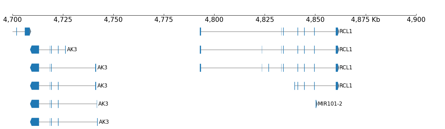
BED track :
BED track is used to show the genome annotation information like RefSeq or chromatin states. Here, we have the RefSeq data which can be visualized with coolbox.api.BED:
Visualizing RefSeq with CoolBox:
[7]:
frame = XAxis() + BED(f"{DATA_DIR}/bed_{RANGE_MARK}.bed") + TrackHeight(8)

frame.plot("chr9:4700000-4900000")
[7]:
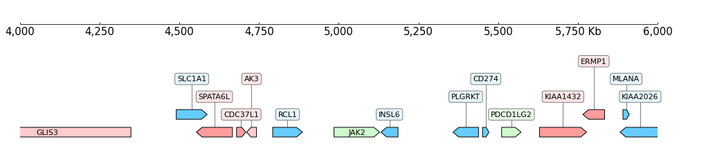
GTFtrack :
GTF track is also used to visualize gene annotations:
[8]:
frame = XAxis() + GTF(f"{DATA_DIR}/gtf_{RANGE_MARK}.gtf") + TrackHeight(5)

frame.plot(TEST_RANGE)
[8]:
Hi-C (.cool) Track
CoolBox also supports Hi-C data visualization.
CoolBox supports two types of input format for Hi-C matrix data, .cool and .hic file.
Their API is very similar, You can use CoolBox.api.HiCMat to visualize both.
Here, we use a .cool file as an example.
multi-cool(.mcool) for multiple resolution Hi-C matrix
Cooler file supports multi-resolution interaction matrix storage (normally file name ends with .mcool), this feature allows us take appropriate resolution matrix data depending on the corresponding genome region size, it lets program respond fast when plotting the Hi-C matrix.
The multi-resolution cooler file is recommended. You can use cooler zoomify command to create multi-resolution cooler file from a single resolution cooler file.
[9]:
frame = XAxis() + HiCMat(f"{DATA_DIR}/cool_{RANGE_MARK}.mcool")
frame.plot(TEST_RANGE)
[9]:
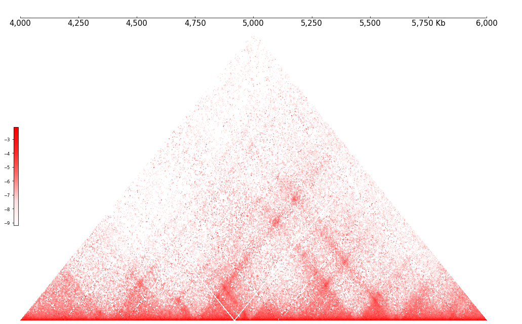
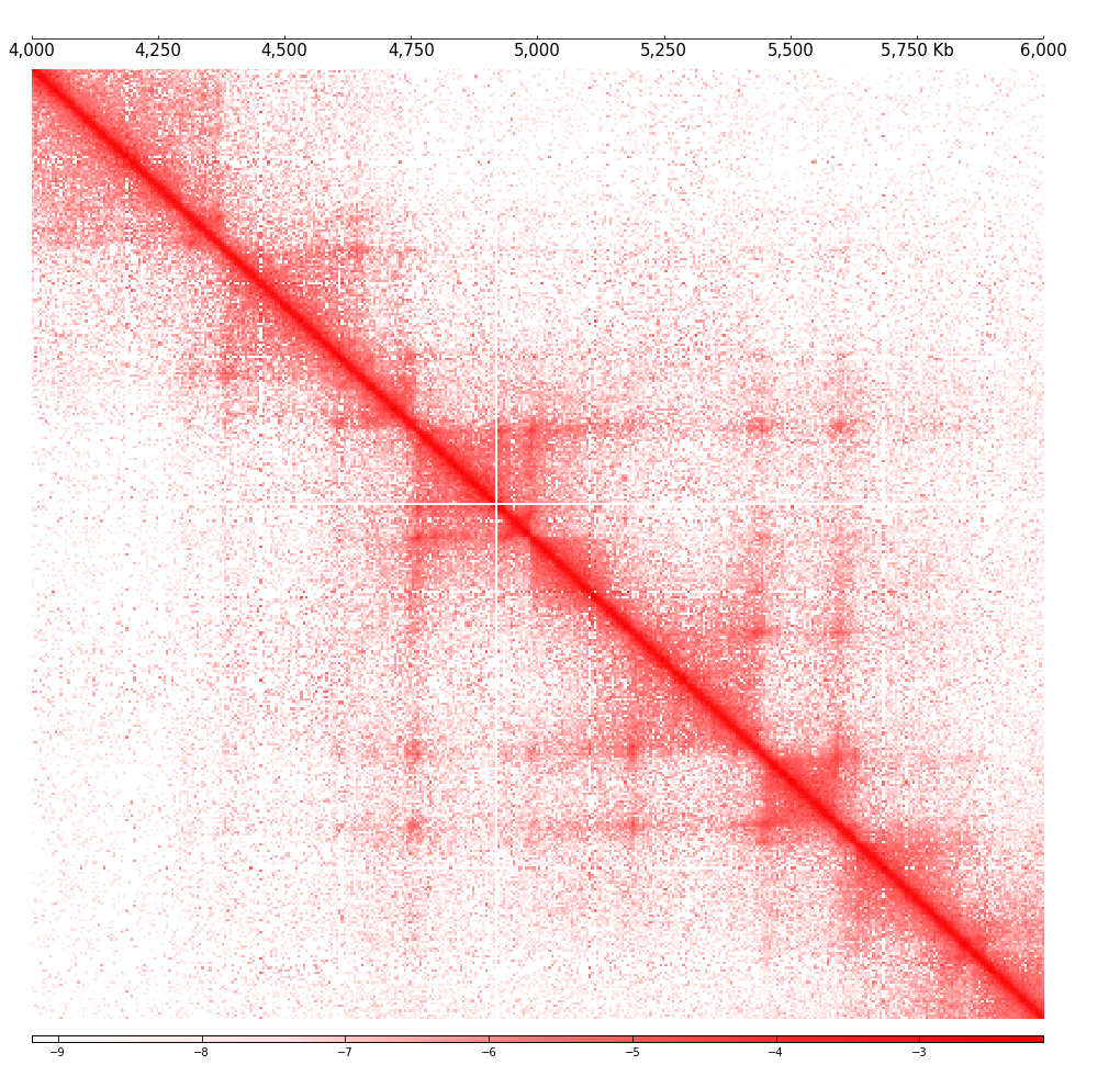
Default Hi-C Track will be plotted in triangular style. It also can be plotted in matrix or window style.
Just specify the style parameter, when creating Cool instance, like this:
[10]:
frame = XAxis() + \
    HiCMat(f"{DATA_DIR}/cool_{RANGE_MARK}.mcool", style='matrix', color_bar='horizontal')
frame.plot(TEST_RANGE)
[10]:
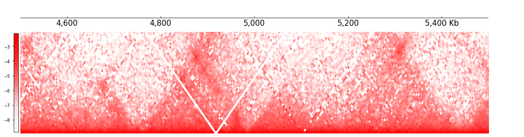
[11]:
frame = XAxis() + HiCMat(f"{DATA_DIR}/cool_{RANGE_MARK}.mcool", style='window', depth_ratio=0.3)
frame.plot("chr9:4500000-5500000")
[11]:
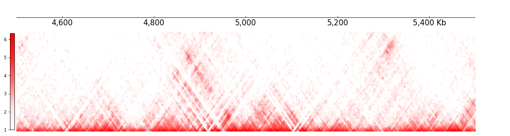
Cool shows balanced matrix as default, if you want to show the unbalanced matrix, you can set as:
[12]:
frame = XAxis() + HiCMat(f"{DATA_DIR}/cool_{RANGE_MARK}.mcool", style='window', depth_ratio=0.3, balance=False) + MinValue(1)
frame.plot("chr9:4500000-5500000")
[12]:
Arcs Track
Technologies like ChIA-PET or HiChIP can produce many long-range genome-wide chromatin interactions.
And, sometimes, the Hi-C contact matrix contains too much information than needed. When we only need some of the most important interactions from it, we can use some tools like HICCUPS to call the most significant interactions, or “peaks” from the contact matrix.
In either case, Arcs Track can be used to visulize the data. Arcs track accepts .pairs or .bedpe format:
[13]:
# BEDPE
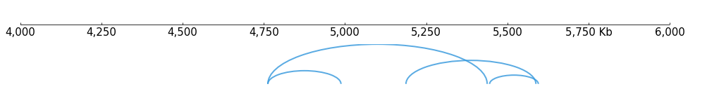
frame = XAxis() + Arcs(f"{DATA_DIR}/bedpe_{RANGE_MARK}.bedpe", line_width=2)
frame.plot(TEST_RANGE)
[13]:
[14]:
# Pairs
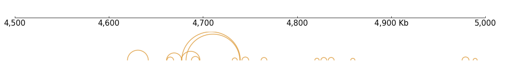
frame = XAxis() + Arcs(f"{DATA_DIR}/pairs_{RANGE_MARK}.pairs", line_width=1.5)
frame.plot("chr9:4500000-5000000")
[14]:
Compose Tracks to Frame
In CoolBox you can compose tracks with “+” operator, as shown above, compose XAxis track and a bigwig track to a frame object:
frame = XAxis() + BigWig("data/K562_RNASeq.bigWig")
Frame is a higher level object and it denotes a set of related tracks. We can use a long “+” expression to compose a complex Frame.
[15]:
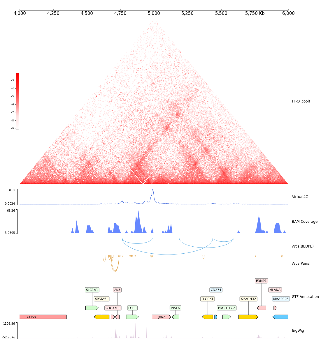
cool1 = Cool(f"{DATA_DIR}/cool_{RANGE_MARK}.mcool")

frame = XAxis() + \
    cool1 + Title("Hi-C(.cool)") + \
    Spacer(0.5) + \
    Virtual4C(cool1, "chr9:4986000-4986000") + Title("Virtual4C") + \
    Spacer(0.5) + \
    BAMCov(f"{DATA_DIR}/bam_{RANGE_MARK}.bam") + Title("BAM Coverage") +\
    Spacer(0.5) + \
    Arcs(f"{DATA_DIR}/bedpe_{RANGE_MARK}.bedpe") + Inverted() + Title("Arcs(BEDPE)") + \
    Spacer(0.1) + \
    Arcs(f"{DATA_DIR}/pairs_{RANGE_MARK}.pairs") + Inverted() + Title("Arcs(Pairs)") + \
    GTF(f"{DATA_DIR}/gtf_{RANGE_MARK}.gtf", length_ratio_thresh=0.005) + TrackHeight(6) + Title("GTF Annotation") + \
    Spacer(0.1) + \
    BigWig(f"{DATA_DIR}/bigwig_{RANGE_MARK}.bw") + Title("BigWig")
[16]:
frame.plot(TEST_RANGE)
[16]:
Adjust Tracks and Frame with Feature
Maybe you have noticed that, in the complex expression above, there are some elements which added with Tracks is not a Track, for example, the TrackHeight, Title and Title.
These elements are Feature and they represent the features of the Track.
For example, we set the color and track height feature of a bigWig track.
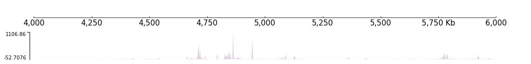
[17]:
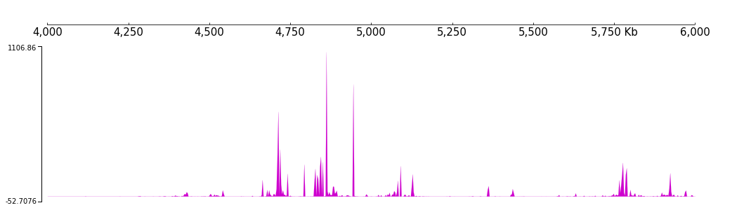
frame = XAxis() + \
        BigWig(f"{DATA_DIR}/bigwig_{RANGE_MARK}.bw") + \
        Color("#ce00ce") + TrackHeight(8)
[18]:
frame.plot(TEST_RANGE)
[18]:
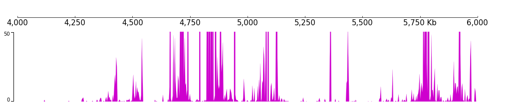
And we can adjust the min value and max value of the track:
[19]:
frame = XAxis() + \
        BigWig(f"{DATA_DIR}/bigwig_{RANGE_MARK}.bw") + \
        Color("#ce00ce") + TrackHeight(5) + \
        MinValue(0) + MaxValue(50)
[20]:
frame.plot(TEST_RANGE)
[20]:
with statement
By the way, there are one useful trick, you can use Feature with “with statement”, like:
[21]:
with Color("#fd9c6b"):
    frame1 = XAxis() +\
             BigWig(f"{DATA_DIR}/bigwig_{RANGE_MARK}.bw") +\
             BigWig(f"{DATA_DIR}/bigwig_{RANGE_MARK}.bw")  +\
             BigWig(f"{DATA_DIR}/bigwig_{RANGE_MARK}.bw")

with Color("#66ccff"):
    frame2 = BigWig(f"{DATA_DIR}/bigwig_{RANGE_MARK}.bw") +\
             BigWig(f"{DATA_DIR}/bigwig_{RANGE_MARK}.bw")

frame = frame1 + frame2
[22]:
frame.plot(TEST_RANGE)
[22]:
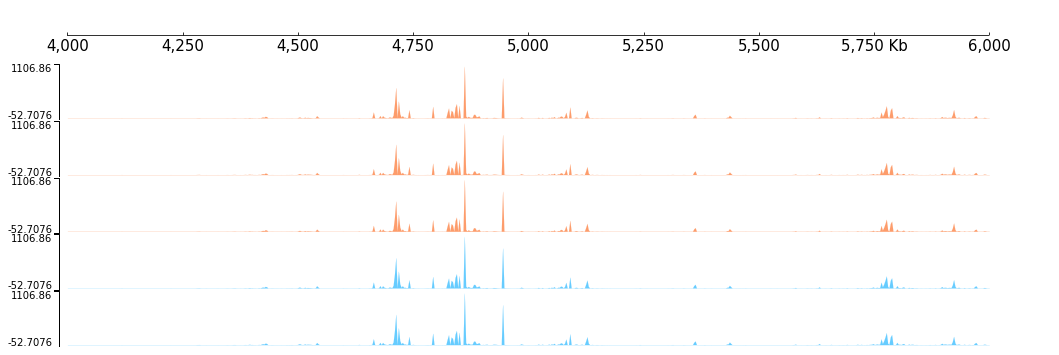
As shown above, any tracks created inside the “with statement” will have the specified feature.
Using this trick, we can simplify the complex expression:
Coverage
Sometimes we need to draw some graphics above the original figure, for example, the vertical lines and highlight regions. CoolBox has another kinds of element, the Coverage. We can add coverage with track, after added to track, coverage will be plotted above the track when the track is plotted.
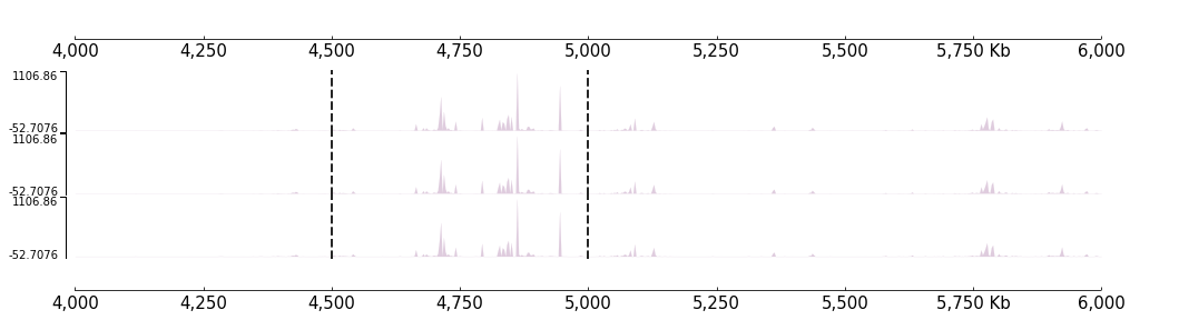
Vertical lines
[23]:
locus = [("chr9", 4500000), ("chr9", 5000000)]
frame = XAxis() + BigWig(f"{DATA_DIR}/bigwig_{RANGE_MARK}.bw") + Vlines(locus, line_width=2)
[24]:
frame.plot(TEST_RANGE)
[24]:

Like the Feature if you want a set of tracks with same coverge, you can use the “with statement”:
[25]:
with Vlines(locus, line_width=2):
    frame = BigWig(f"{DATA_DIR}/bigwig_{RANGE_MARK}.bw") +\
            BigWig(f"{DATA_DIR}/bigwig_{RANGE_MARK}.bw") +\
            BigWig(f"{DATA_DIR}/bigwig_{RANGE_MARK}.bw")
frame = XAxis() + frame + XAxis()
[26]:
frame.plot(TEST_RANGE)
[26]:
Or, you can also use * operator do this:
[27]:
frame = BigWig(f"{DATA_DIR}/bigwig_{RANGE_MARK}.bw") +\
        BigWig(f"{DATA_DIR}/bigwig_{RANGE_MARK}.bw") +\
        BigWig(f"{DATA_DIR}/bigwig_{RANGE_MARK}.bw")
frame = frame * Vlines(locus, line_width=2)
frame = XAxis() + frame + XAxis()
[28]:
frame.plot(TEST_RANGE)
[28]:

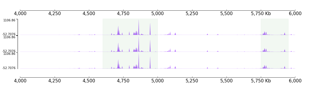
HighLights
[29]:
regions= ["chr9:4600000-5000000", "chr9:5750000-5950000"]

highlights = HighLights(regions, color="green", alpha=0.05)

with highlights, Color("#aa5cff"):
    frame = BigWig(f"{DATA_DIR}/bigwig_{RANGE_MARK}.bw") +\
            BigWig(f"{DATA_DIR}/bigwig_{RANGE_MARK}.bw") +\
            BigWig(f"{DATA_DIR}/bigwig_{RANGE_MARK}.bw")

frame = XAxis() + frame + XAxis()
[30]:
frame.plot(TEST_RANGE)
[30]:
Explore Genomic Data with coolbox.api.Browser
When you want to explore the data, you will change the genome region window very frequently. Under these circumstances, when you want to do the operations like “move right”, “move left”, “zoom in”, “zoom out”, if you use above Frame.plot API to plot the figure, you must change parameters and run again. It is tiresome and boring. In order to solve this problem, CoolBox impletmented a simple GUI with ipywidgets.
You can create a Browser instance with a composed frame, and call .show() method to show the browser.
[31]:
cool1 = Cool(f"{DATA_DIR}/cool_{RANGE_MARK}.mcool")

frame = XAxis() + \
    cool1 + Title("Hi-C(.cool)") + \
    Spacer(0.5) + \
    Virtual4C(cool1, "chr9:4986000-4986000") + Title("Virtual4C") + \
    Spacer(0.5) + \
    BAM(f"{DATA_DIR}/bam_{RANGE_MARK}.bam") + Title("BAM Coverage") +\
    Spacer(0.5) + \
    Arcs(f"{DATA_DIR}/bedpe_{RANGE_MARK}.bedpe") + Inverted() + Title("Arcs(BEDPE)") + \
    Spacer(0.1) + \
    Arcs(f"{DATA_DIR}/pairs_{RANGE_MARK}.pairs") + Inverted() + Title("Arcs(Pairs)") + \
    GTF(f"{DATA_DIR}/gtf_{RANGE_MARK}.gtf", length_ratio_thresh=0.005) + TrackHeight(6) + Title("GTF Annotation") + \
    Spacer(0.1) + \
    BigWig(f"{DATA_DIR}/bigwig_{RANGE_MARK}.bw") + Title("BigWig")

bsr = Browser(frame)
bsr.goto(TEST_RANGE)
Note: browser is valid only when the jupyter kernel is active
[32]:
bsr.show()
Fetch precise data use .fetch_data API
In CoolBox, data and figure are bound together with a single Python object. So, you can fetch precise data of what you see in the figure.
Call the .fetch_data method of Browser or Frame, will return an collection.OrderDict which stores many pandas.Dataframe objects corresponding to each track in the browser or frame, and the data is only about the current genome region.
[33]:
bsr.tracks
[33]:
OrderedDict([('XAxis.21', <coolbox.core.track.pseudo.XAxis at 0x758abb46f5c0>),
             ('Cool.6',
              <coolbox.core.track.hicmat.cool.Cool at 0x758abba161e0>),
             ('Spacer.6',
              <coolbox.core.track.pseudo.Spacer at 0x758abb32f140>),
             ('Virtual4C.2',
              <coolbox.core.track.hist.hicfeature.Virtual4C at 0x758abb949280>),
             ('Spacer.7',
              <coolbox.core.track.pseudo.Spacer at 0x758abbf8d3d0>),
             ('BAM.1', <coolbox.core.track.bam.BAM at 0x758abb3b97f0>),
             ('Spacer.8',
              <coolbox.core.track.pseudo.Spacer at 0x758ac03546b0>),
             ('BEDPE.3',
              <coolbox.core.track.arcs.bedpe.BEDPE at 0x758abb6ecc20>),
             ('Spacer.9',
              <coolbox.core.track.pseudo.Spacer at 0x758abbc1c0e0>),
             ('Pairs.3',
              <coolbox.core.track.arcs.pairs.Pairs at 0x758abb882180>),
             ('GTF.3', <coolbox.core.track.gtf.GTF at 0x758abb6816d0>),
             ('Spacer.10',
              <coolbox.core.track.pseudo.Spacer at 0x758abb354800>),
             ('BigWig.20',
              <coolbox.core.track.hist.bigwig.BigWig at 0x758ac0bfca40>)])
[34]:
current_data = bsr.fetch_data()
[35]:
list(current_data.keys())
[35]:
['XAxis.21',
 'Cool.6',
 'Spacer.6',
 'Virtual4C.2',
 'Spacer.7',
 'BAM.1',
 'Spacer.8',
 'BEDPE.3',
 'Spacer.9',
 'Pairs.3',
 'GTF.3',
 'Spacer.10',
 'BigWig.20']
Data of each track related to the current genome range are stored in this dict:
[36]:
current_cool = current_data['Cool.6']
[37]:
print(type(current_cool))
current_cool.shape
<class 'numpy.ndarray'>
[37]:
(401, 401)
[38]:
current_data['GTF.3'].head(5)
[38]:
| seqname | source | type | start | end | score | strand | frame | attributes | feature_name | |
|---|---|---|---|---|---|---|---|---|---|---|
| 0 | chr9 | protein_coding | gene | 3824127 | 4348392 | NaN | - | NaN | gene_biotype "protein_coding"; gene_id "ENSG00... | GLIS3 |
| 1 | chr9 | protein_coding | transcript | 3824127 | 4152183 | NaN | - | NaN | ccds_id "CCDS6451"; gene_biotype "protein_codi... | GLIS3 |
| 2 | chr9 | protein_coding | transcript | 3827698 | 4299916 | NaN | - | NaN | ccds_id "CCDS43784"; gene_biotype "protein_cod... | GLIS3 |
| 3 | chr9 | retained_intron | transcript | 3855437 | 4118017 | NaN | - | NaN | gene_biotype "protein_coding"; gene_id "ENSG00... | GLIS3 |
| 4 | chr9 | processed_transcript | transcript | 3932360 | 4081361 | NaN | - | NaN | gene_biotype "protein_coding"; gene_id "ENSG00... | GLIS3 |
We can perform some statistics analysis on it. For example, count the distribution of interaction count, etc…
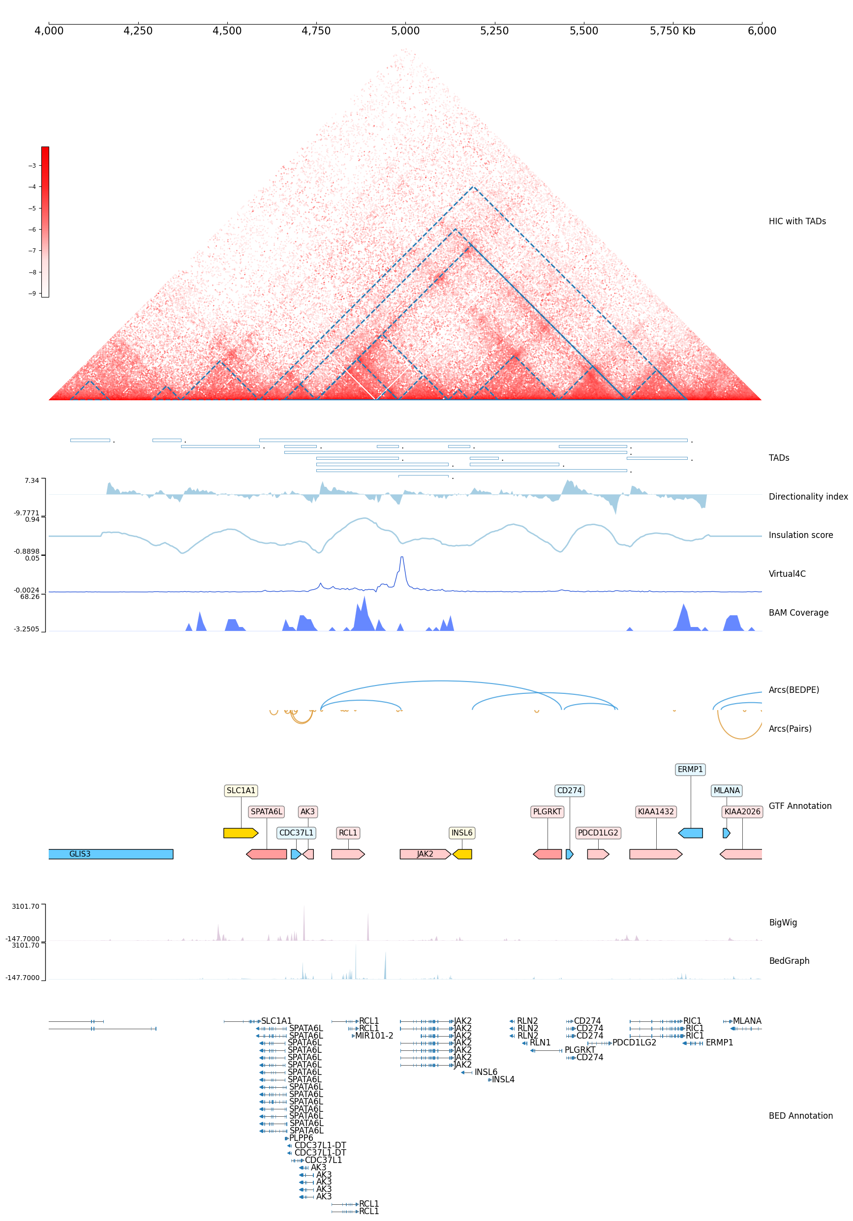
Taken together
[39]:
DATA_DIR = f"tests/test_data"
test_interval = "chr9:4000000-6000000"
test_itv = test_interval.replace(':', '_').replace('-', '_')

cool1 = Cool(f"{DATA_DIR}/cool_{test_itv}.mcool", cmap="JuiceBoxLike", style='window', color_bar='vertical')
with TrackHeight(2):
    frame = XAxis() + \
        cool1 + Title("Hi-C(.cool)") + \
        TADCoverage(f"{DATA_DIR}/tad_{test_itv}.bed", border_only=True, alpha=1) + Title("HIC with TADs") + \
        Spacer(0.1) + \
        BED(f"{DATA_DIR}/tad_{test_itv}.bed", border_only=True, alpha=1) + Title("TADs") + \
        DiScore(cool1, window_size=30) + Feature(title="Directionality index") + \
        InsuScore(cool1, window_size=30) + Title("Insulation score") + \
        Virtual4C(cool1, "chr9:4986000-4986000") + Title("Virtual4C") + \
        BAMCov(f"{DATA_DIR}/bam_{test_itv}.bam") + Title("BAM Coverage") +\
        Spacer(0.1) + \
        Arcs(f"{DATA_DIR}/bedpe_{test_itv}.bedpe", line_width=1.5) + Title("Arcs(BEDPE)") + \
        Arcs(f"{DATA_DIR}/pairs_{test_itv}.pairs", line_width=1.5) + Inverted() + Title("Arcs(Pairs)") + \
        GTF(f"{DATA_DIR}/gtf_{test_itv}.gtf", length_ratio_thresh=0.005) + TrackHeight(6) + Title("GTF Annotation") + \
        Spacer(0.1) + \
        BigWig(f"{DATA_DIR}/bigwig_{test_itv}.bw") + Title("BigWig") + \
        BedGraph(f"{DATA_DIR}/bedgraph_{test_itv}.bg") + Title("BedGraph") + \
        Spacer(0.1) + \
        BED(f"{DATA_DIR}/bed_{test_itv}.bed") + Feature(height=10, title="BED Annotation")
frame.properties['width'] = 45
frame.goto(test_interval)
frame.show()
[39]: